How Can Randomized Smoothing Adapt? Neural Network Certification, Part 9
On this page
Certification Series
April’s photographs do not all need the same treatment
Part 8 built a smoothed classifier by adding Gaussian noise, asking a base classifier for labels, and taking the most probable label. Its certificate came from a fixed noise level $\sigma$.
Now place two April photographs beside that pipeline. The classifier’s noisy votes around one image are fragile, while its votes around the other remain stable under stronger perturbations. The same base model and the same $\sigma$ process both images.
The contrast raises a new question:
Which parts of randomized smoothing can adapt to the model or the input without breaking the certificate?
We will change two components. Denoised smoothing changes the function that receives the noisy input. Input-dependent smoothing changes the noise level itself.
A denoiser can stand in front of a pretrained classifier
Part 8 defined randomized smoothing by drawing $\eta\sim\mathcal N(0,\sigma^2I)$ and predicting the class most likely under $x+\eta$. A radius $R$ certifies that this prediction cannot change for any $x’$ with $\lVert x’-x\rVert_2<R$. If $\underline p_A>1/2$ is a statistically valid lower bound on the winning-class probability, the common finite-sample certificate is
\[R=\sigma\Phi^{-1}(\underline p_A),\]where $\Phi^{-1}$ is the inverse standard-normal cumulative distribution function.
Let $D$ be a denoiser and $f$ a classifier. Denoised smoothing inserts $D$ between the noisy input and $f$:
\[x+\eta \longrightarrow D(x+\eta) \longrightarrow f(D(x+\eta)).\]The composition
\[h=f\circ D\]is simply another base classifier. The smoothing theorem from Part 8 allowed the base classifier to be any function, so we can define
\[g_D(x)=\arg\max_c \Pr\bigl(f(D(x+\eta))=c\bigr)\]and apply the same Gaussian radius formula.
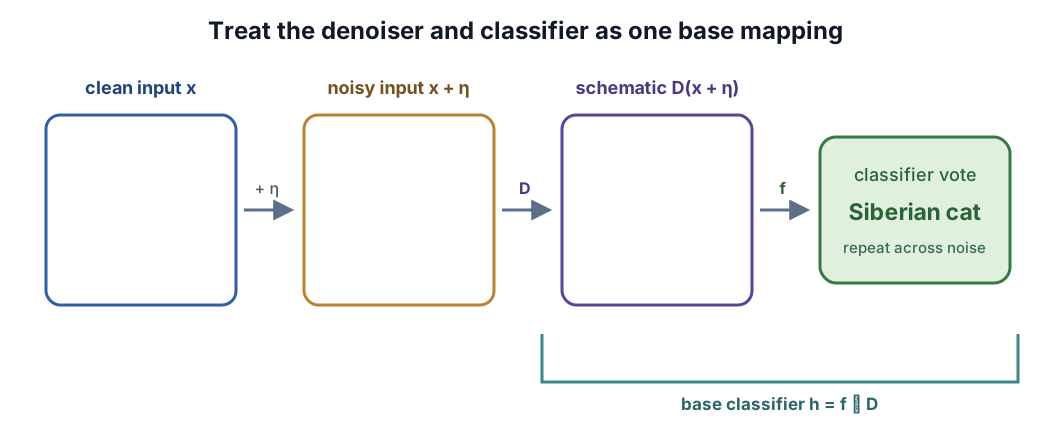
Denoised smoothing trains $D$ so that noisy images recover features useful to an existing classifier. The classifier’s parameters can remain fixed, which makes it possible to add a certified robustness wrapper around a pretrained or even black-box image service.
The certificate depends on how large the winning-class probability is for the composed classifier $f\circ D$ across the Gaussian cloud.
The source of the denoiser is therefore a practical design choice. Can we reuse a pretrained model that already knows how to remove image noise?
Reuse an off-the-shelf denoiser
A diffusion model learns to reverse a gradual noising process, so it can fill the denoising position in the pipeline above.
The method (Certified!!) Adversarial Robustness for Free! combines a pretrained diffusion model with a pretrained image classifier. For each Gaussian-perturbed input, the diffusion model performs a denoising step and the classifier supplies a vote. The published construction requires no fine-tuning of either pretrained model.
The method matches $\sigma$ to a diffusion timestep, rescales the noisy image, and performs one denoising step before classification. The resulting denoiser and classifier form the base mapping, so the ordinary smoothing theorem still converts its noisy votes into an $\ell_2$ certificate.
Denoising adapts the base mapping while keeping one global noise level. The second kind of adaptation changes the noise scale itself.
One global noise level creates conflicting goals
The noise scale $\sigma$ appears both in the data distribution and in the radius:
\[R=\sigma\Phi^{-1}(p_A)\]for the common one-probability form of the certificate.
A smaller $\sigma$ perturbs April’s image less, so the winning class often has a higher probability $p_A$. A larger $\sigma$ widens the Gaussian cloud and multiplies the quantile, but $p_A$ may fall. Different inputs maximize $R(\sigma)$ at different noise scales depending on their stability under perturbations.
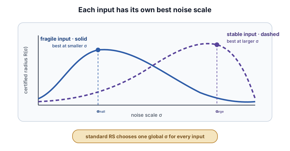
For each photograph, we would therefore like to select the noise level that gives the most useful certificate.
Why can we not substitute an arbitrary $\sigma(x)$?
The standard proof compares the Gaussian distribution centered at $x$ with the same distribution shifted to $x+\delta$. A global $\sigma$ ensures that only the center moves.
If we replace $\sigma$ with an arbitrary function $\sigma(x)$, a nearby input may change both the center and the spread:
\[\mathcal N(x,\sigma(x)^2I) \quad\hbox{versus}\quad \mathcal N(x+\delta,\sigma(x+\delta)^2I).\]The Part 8 theorem does not compare these two distributions. A method that chooses a useful noise scale per test point therefore needs an argument connecting the choices at neighboring points.
Data-dependent randomized smoothing chooses $\sigma$ per query and stores previously certified regions. Its memory-based procedure adjusts predictions or shrinks regions to prevent overlapping certified regions from carrying different labels.
A later analysis of input-dependent smoothing formalizes why rapidly changing noise-scale functions cannot inherit the ordinary certificate and studies conditions that restore a sound guarantee.
Local constancy supplies the missing connection
Suppose a scale selector chooses $\sigma(x)$ and remains constant throughout a ball around $x$:
\[\sigma(x')=\sigma(x) \qquad\text{for every }x'\text{ with } \lVert x'-x\rVert_2<R_\sigma.\]Inside that ball, all inputs invoke the same Gaussian noise scale. The standard smoothing comparison is available again.
The Dual Randomized Smoothing theorem states this requirement precisely. If the scale selector is constant on $B(x,R_\sigma)$, and ordinary smoothing at the selected scale certifies $R_c$, the adaptive classifier is certified to $\min(R_\sigma,R_c)$. In practice, both the constancy claim and the class-probability claim are estimated statistically. If their failure probabilities are $\alpha_\sigma$ and $\alpha_c$, the union bound gives joint confidence at least
\[1-(\alpha_\sigma+\alpha_c).\]No independence assumption is needed for that confidence calculation.
The theorem leaves an implementation question: how can one system certify the selector and the selected classifier for the same input?
Dual randomized smoothing certifies the selector and the prediction
Dual randomized smoothing (Dual RS) implements the idea with two smoothed models.
- The paper’s variance estimator predicts one noise standard deviation $\sigma$ from a finite set such as ${0.25,0.5,1.0}$. The estimator itself is smoothed, so it returns both a selected scale and a radius $R_\sigma$ within which that selection cannot change.
- A classification model is smoothed with the selected scale. It returns April’s label and a classification radius $R_c$.
The final certified radius is
\[R=\min(R_\sigma,R_c).\]The minimum has a direct meaning. Before reaching $R_\sigma$, the route stays on the same noise level. Before reaching $R_c$, that route’s smoothed classifier keeps the same label. Staying inside both radii preserves the entire two-stage decision.
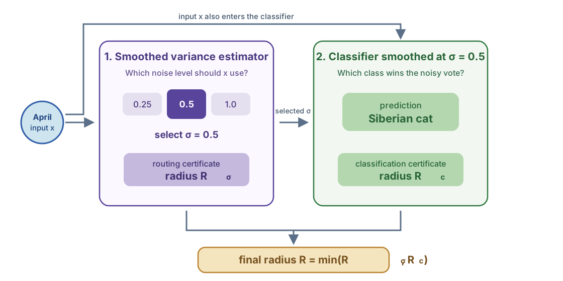
The estimator can also route inputs among pretrained randomized-smoothing experts, each specialized for one noise scale. Improving an expert can improve certificates for inputs routed to it after recertification, without changing the soundness argument.
Two kinds of adaptation, one proof discipline
The two method families change different parts of randomized smoothing.
| What adapts? | Example | Why the certificate remains valid |
|---|---|---|
| The base mapping becomes $f\circ D$. | Diffusion denoised smoothing supplies a pretrained $D$. | The smoothing theorem permits any base classifier. |
| The noise scale becomes $\sigma(x)$. | Dual RS certifies a selector over scales or experts. | Local constancy is certified first. The selected classifier is certified second. |
The two routes are sound for different reasons: denoised smoothing changes the base mapping while keeping the theorem applicable, whereas input-dependent smoothing certifies the selector before using its chosen noise scale.
Certification is a discipline of complete coverage
Part 1 began with a gap between testing some inputs and proving a claim for every allowed input. Across the series, we followed two routes to close that gap.
Deterministic verification covers every possible ReLU phase with sound bounds and, when needed, branches. Denoised smoothing makes a fixed denoiser part of the base mapping, which the smoothing theorem already covers. Input-dependent smoothing adds an adaptive selector, whose local constancy requires its own certificate before the selected noise scale or expert can be used.
Neural network certification is therefore a discipline of complete coverage. The mathematical tools change, while the central question remains: which allowed inputs and model behaviors does this argument cover?