How Can Random Noise Produce a Certificate? Neural Network Certification, Part 8

On this page

Certification Series

One photograph of April becomes a cloud

The deterministic methods in Parts 2 through 6 tracked every allowed perturbation through every network layer. Randomized smoothing takes a different route: it treats a neural network as a black box and certifies a new classifier built from its noisy votes.

We now leave April’s two-class teaching model and let the black-box base classifier use a richer label set: Siberian cat, tree, and other animal.

Start with April’s photograph. Add independent Gaussian noise to every pixel, classify each noisy copy, and count the labels. Some copies may look grainy, but suppose “Siberian cat” wins a large majority.

This creates the central question:

How can agreement across random noisy inputs guarantee the prediction for every adversarial input inside a fixed radius?

Build a new classifier from noisy votes

Let $f$ be any base classifier and let

\[\eta\sim\mathcal N(0,\sigma^2I).\]

The vector $\eta$ contains one independent Gaussian noise value per input coordinate, and $I$ is the identity matrix. The parameter $\sigma$ is the noise standard deviation: larger $\sigma$ creates a wider cloud around the original input.

The smoothed classifier is

\[g(x)=\arg\max_c\Pr\bigl(f(x+\eta)=c\bigr).\]

Read the formula from the inside out:

1. sample a noisy input $x+\eta$.
2. ask the base classifier $f$ for its label.
3. compute the probability of each class across the noise.
4. let $g$ return the most probable class.

The classifier being certified is $g$. The base classifier $f$ supplies the votes.

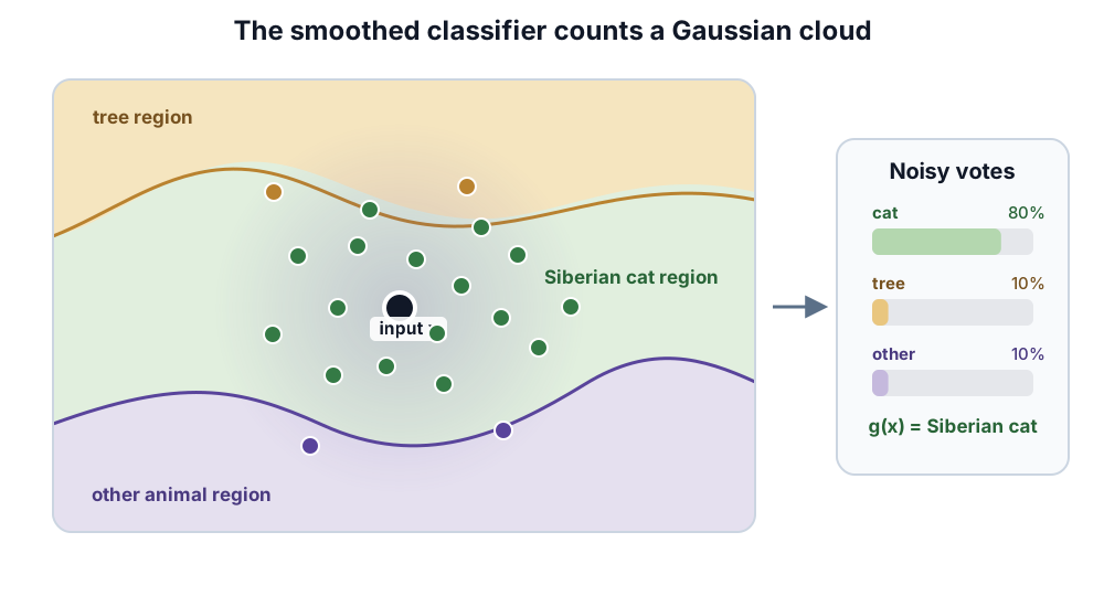
The vote identifies the smoothed label. Certification must also convert that label’s probability lead into a distance around April’s input.

A probability gap becomes a certified radius

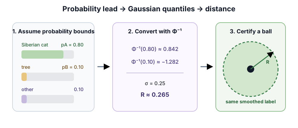
The 20 dots above illustrate a Gaussian cloud. Their visible frequencies are not probability estimates for certification. For the idealized calculation below, assume the exact class probabilities admit the bounds $p_A=0.80$ and $p_B=0.10$. A finite-sample certificate will replace those assumed bounds with statistical confidence bounds in the next section.

Let $c_A$ be the most probable class. Suppose we know

\[\Pr(f(x+\eta)=c_A)\geq p_A\]

and every competing class has probability at most $p_B$, with $p_A>p_B$. For Gaussian noise, the randomized smoothing theorem gives the radius

\[R=\frac{\sigma}{2} \left(\Phi^{-1}(p_A)-\Phi^{-1}(p_B)\right),\]

where $\Phi$ is the cumulative distribution function of a standard normal random variable. Its inverse $\Phi^{-1}(p)$ converts a probability into the corresponding position on the normal curve.

The full formula uses both the leading-class lower bound $p_A$ and a competitor upper bound $p_B$. A common certificate uses only $p_A$. All competing classes together have probability at most $1-p_A$, so every single competitor also has probability at most

\[p_B\leq 1-p_A.\]

The inequality above is the common relaxed competitor bound. It treats all probability outside $c_A$ as though one hypothetical competitor owns it, so it requires no separate estimate of the runner-up class.

Substituting the valid choice $p_B=1-p_A$ into the two-probability formula and using $\Phi^{-1}(1-p)=-\Phi^{-1}(p)$ gives

\[R_A=\sigma\Phi^{-1}(p_A), \qquad p_A>\frac12.\]

The resulting formula is the common one-probability certificate, and it remains valid for any number of classes. When a separately computed $p_B$ is smaller than $1-p_A$, the two-probability formula uses that extra information to certify a larger radius. The Monte Carlo procedure below will estimate a lower bound on $p_A$ and substitute it into this one-probability formula.

An adversarial input is $x+\delta$, deliberately chosen subject to a norm limit. The theorem states that

\[\lVert\delta\rVert_2<R \quad\Longrightarrow\quad g(x+\delta)=c_A.\]

One probability calculation therefore covers every perturbation $\delta$ inside an $\ell_2$ ball: all changes whose total Euclidean length is below $R$.

Assume pixel coordinates are scaled to $[0,1]$, so $\sigma$ and $R$ use those normalized units. For this idealized example, take $\sigma=0.25$, $p_A=0.80$, and $p_B=0.10$. Since

\[\Phi^{-1}(0.80)\approx0.842, \qquad \Phi^{-1}(0.10)\approx-1.282,\]

the certified radius is

\[R\approx\frac{0.25}{2}(0.842+1.282)=0.265.\]

If only $p_A=0.80$ is available, every competitor is instead bounded by $1-p_A=0.20$. The one-probability radius is

\[R_A=0.25\Phi^{-1}(0.80)\approx0.210.\]

Both radii are sound. The first uses the additional fact that the strongest competitor has probability at most $0.10$, while the second needs only the leading-class probability.

To see why these formulas cover a whole ball, write $r=\lVert\delta\rVert_2$. After the Gaussian center moves by $\delta$, the leading-class probability is at least

\[\Phi\!\left(\Phi^{-1}(p_A)-\frac r\sigma\right),\]

while any competitor’s probability is at most

\[\Phi\!\left(\Phi^{-1}(p_B)+\frac r\sigma\right).\]

The leading-class lower bound remains larger than the competitor upper bound whenever $r<\frac{\sigma}{2}(\Phi^{-1}(p_A)-\Phi^{-1}(p_B))$. The Neyman–Pearson lemma justifies these worst-case bounds: among decision regions with the stated original probability, a half-space perpendicular to $\delta$ changes the most when the Gaussian center shifts.

For the one-probability certificate, substitute $p_B=1-p_A$. The competitor’s shifted upper bound becomes

\[\Phi\!\left(\Phi^{-1}(1-p_A)+\frac r\sigma\right).\]

The leading-class lower bound stays larger precisely while $r<\sigma\Phi^{-1}(p_A)$, recovering $R_A$ above.

Where does probability enter the certificate?

Probability enters the certificate in two different ways, and separating them prevents a common misreading.

First, Gaussian noise defines the mathematical smoothed classifier $g$. If its class probabilities were known exactly, the radius theorem would make a deterministic statement: every input in the ball receives the same label from $g$.

Second, a computer cannot evaluate the exact probabilities of a modern neural network. A sound finite-sample procedure therefore separates selection from estimation:

1. Use a pilot batch of noisy inputs to choose a candidate class $c_A$.
2. Use a fresh, larger batch to compute a one-sided confidence lower bound $\underline p_A$ for that class.
3. Use $1-\underline p_A$ as an upper bound for every competing class.
4. Return $R=\sigma\Phi^{-1}(\underline p_A)$ when $\underline p_A>1/2$, and abstain otherwise.

The procedure is the finite-sample form of the one-probability certificate above. A confidence lower bound replaces the ideal $p_A$, so sampling uncertainty stays inside the stated guarantee. Choose the one-sided bound with failure probability $\alpha$.

The practical certificate therefore says:

With probability at least $1-\alpha$ over the Monte Carlo samples, the returned label-radius pair is valid.

The noisy samples here are evaluation samples, not attack samples. They estimate a probability under the specified Gaussian distribution. A statistical confidence bound on that probability, combined with the analytic smoothing theorem, covers every adversarial perturbation in the certified ball. The failure probability $\alpha$ belongs to the Monte Carlo certification procedure.

The algorithm either returns this radius or abstains. A narrow vote margin may identify the winning class while providing insufficient statistical evidence for a positive radius. Abstention keeps sampling uncertainty inside the stated guarantee.

This procedure certifies a fixed base classifier. Obtaining a useful radius also requires that classifier to give the correct class a large probability advantage under Gaussian noise.

How should the base classifier be trained?

At a fixed noise level $\sigma$, the radius grows when the correct class remains highly probable under Gaussian noise. Training methods differ in how they create that probability advantage.

Three broad strategies appear repeatedly:

• Learn from Gaussian noise. Ordinary Gaussian training teaches $f$ on the same noisy inputs used at certification time.
• Directly enlarge the useful vote or radius margin. MACER optimizes a radius-based objective, while Consistency encourages noisy copies to produce similar predictions.
• Emphasize difficult or uncertain inputs. SmoothAdv searches for perturbations that weaken the noisy vote. SmoothMix mixes examples along such directions. CAT-RS adjusts the training pressure using confidence.

These methods modify training. The certificate is still computed afterward from noisy class probabilities and the smoothing theorem. This mirrors Part 6: the training signal and the final evaluation guarantee are separate objects.

Once training changes the vote probabilities, we need a dataset-level measure to decide whether robustness improved. A common choice is average certified radius.

Why can average certified radius reward the wrong progress?

For each dataset input, the smoothed classifier may return the correct label, an incorrect label, or abstain. A common summary is the average certified radius (ACR): add the radii of correctly classified inputs, assign radius zero to misclassified or abstained inputs, and divide by the dataset size.

An average hides how the radii are distributed. More subtly, the ideal radius

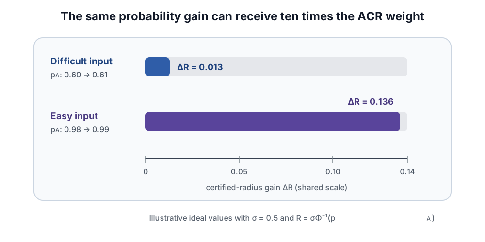
\[R=\sigma\Phi^{-1}(p_A)\]

for the common one-probability certificate is highly nonlinear in $p_A$. Improving an already easy input can change the radius much more than the same probability improvement on a hard input.

Here $p_A$ means the top-class noisy-vote probability. To isolate the formula’s nonlinearity, ignore sampling for this numerical comparison. Take $\sigma=0.5$. Increasing $p_A$ from $0.60$ to $0.61$ changes the ideal radius from about $0.127$ to $0.140$, a gain of $0.013$. Increasing $p_A$ from $0.98$ to $0.99$ changes it from about $1.027$ to $1.163$, a gain of $0.136$. Both probability improvements are $0.01$. The easy input contributes more than ten times as much radius gain.

The paper “Average Certified Radius is a Poor Metric for Randomized Smoothing” proves stronger results. With a large enough sampling budget, a classifier that always predicts one class can obtain arbitrarily large ACR. Under common budgets, ACR is extremely sensitive to easy samples and can change method rankings when the budget changes. The study also finds that several training methods with improved ACR reduce noisy accuracy on hard samples relative to Gaussian training.

A more informative evaluation retains the distribution. Two useful views are:

• certified accuracy at radius $r$: the fraction of the dataset that is correctly certified at least up to $r$, plotted for many radii.
• the empirical distribution of $p_A$: how noisy accuracy is spread across easy and difficult inputs.

Actual ACR replaces the ideal probabilities in our calculation with confidence bounds, so it also depends on the sample count and confidence level. The curves reveal whether progress reaches many inputs, including difficult ones, or mostly extends radii that were already large.

From noisy votes to a probabilistic certificate

The pieces form one chain:

\[\text{base classifier} \longrightarrow \text{Gaussian noisy votes} \longrightarrow \text{confidence bounds} \longrightarrow \text{certified radius or abstention}.\]

The smoothing theorem converts a probability gap into an $\ell_2$ radius. Finite sampling adds an explicit confidence level. Training shapes the probability gap, and evaluation should show how the resulting robustness is distributed across inputs.

Part 9 will adapt two components of this chain. A denoiser will change how the base classifier sees noisy inputs, and a certified selector will let different inputs use different noise levels.