How Can Training Make Robustness Easier to Prove? Neural Network Certification, Part 6

On this page

Certification Series

April is robust, yet the proof took work

Part 5 proved that April’s tiny classifier is robust at radius $0.24$. Its exact worst margin is $0.22$. A single DeepPoly pass gave the inconclusive lower bound $-0.02$, so the verifier had to split the input region before the proof became clear.

The classifier already made the right prediction throughout the region. Its parameters made that fact difficult for a fast bound to establish. Training therefore has a second goal beyond fitting the data: can it learn a robust classifier whose robustness is also easy to prove?

The target is the worst loss in the allowed region

Let $\theta$ collect all trainable weights and biases. For an allowed input $x’\in S$, write the cat-versus-other margin as $m_\theta(x’)$. We will use the binary cross-entropy loss

\[\ell(m)=\log(1+e^{-m}).\]

A larger margin gives a smaller loss. Ordinary training minimizes the loss at the original input $x$:

\[L_{\mathrm{clean}}(\theta)=\ell(m_\theta(x)).\]

Robust training cares about the hardest allowed input, so its ideal target is

\[L_{\mathrm{worst}}(\theta) =\max_{x'\in S}\ell(m_\theta(x')).\]

Computing this maximum exactly for every training example and every parameter update would require solving a verification problem inside each training step. Training methods therefore replace it with a tractable signal that approximates the same target.

Attacks and certificates bracket the target

An attack finds one allowed input $x_{\mathrm{adv}}$ with a large loss. Its training signal is

\[L_{\mathrm{attack}}(\theta) =\ell(m_\theta(x_{\mathrm{adv}})).\]

Because $x_{\mathrm{adv}}$ is one candidate in the maximization, $L_{\mathrm{attack}}$ is a lower bound on the exact worst-case loss.

A sound bound-propagation method covers the whole region. Suppose it returns a sound lower bound

\[\underline m_\theta\leq\min_{x'\in S}m_\theta(x').\]

Since $\ell$ decreases as the margin grows, the certified loss

\[L_{\mathrm{cert}}(\theta)=\ell(\underline m_\theta)\]

is an upper bound on the exact worst-case loss. The three quantities obey

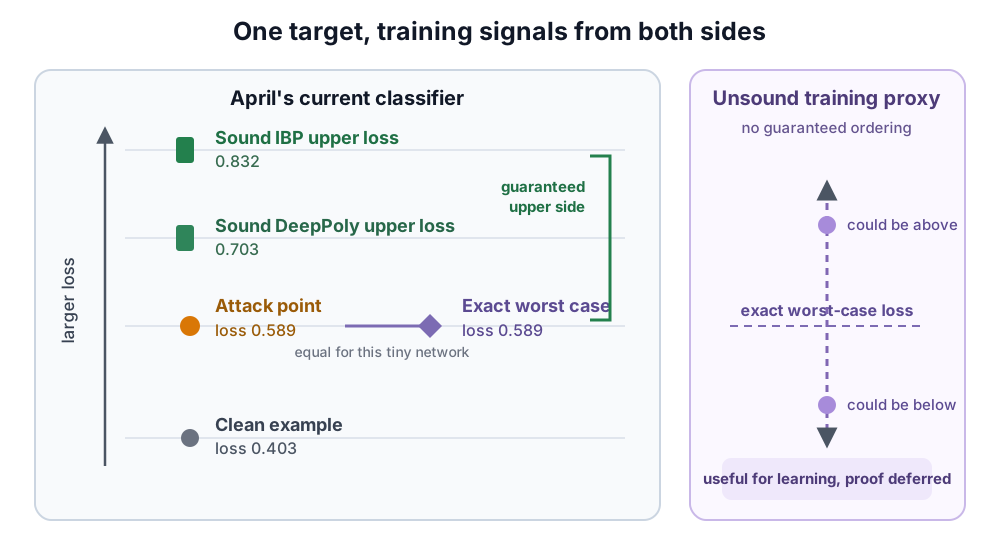
\[\boxed{ L_{\mathrm{attack}}(\theta) \leq L_{\mathrm{worst}}(\theta) \leq L_{\mathrm{cert}}(\theta) }.\]

The attack supplies a concrete hard example. The sound bound supplies coverage of the entire allowed region. The middle quantity is the exact training target.

Put April’s numbers on the bracket

At the center $x=(0.5,0.5)$, April’s margin is $0.70$, giving $L_{\mathrm{clean}}\approx0.403$. An attack can reach $(0.26,0.26)$, where the margin is $0.22$ and the loss is approximately $0.589$. Part 5’s exact proof confirms that this point attains the worst-case margin.

The sound DeepPoly lower margin $-0.02$ gives $L_{\mathrm{cert}}\approx0.703$. At the same radius, IBP gives $h_1\in[0.02,0.98]$ and $h_2\in[0,0.48]$, so its independent intervals yield

\[m\geq0.2+0.02-0.48=-0.26.\]

This coarser margin gives the larger certified loss $0.832$. Both certified losses safely cover the exact worst-case loss.

Sound certified training follows the upper bound

A sound certified-training objective uses a guaranteed full-region upper bound as its robust training signal. Averaging over labeled training examples $(x,y)$ gives

\[\min_\theta\;\mathbb{E}_{(x,y)} \left[L_{\mathrm{cert}}(\theta;x,y)\right].\]

The bound is recomputed after each parameter update because changing $\theta$ changes both the network and its certificate. A minimal training step is:

1. Take a batch of labeled examples.
2. Build the allowed region $S_p(x,\epsilon)$ around each example according to the chosen norm $p$ and radius $\epsilon$.
3. Propagate sound bounds through the current network.
4. Convert the resulting margin bounds into $L_{\mathrm{cert}}$.
5. Differentiate that loss and update $\theta$.

Optimizing this bound can improve the network’s true margins and reshape the network so that bound propagation loses less information. Two common sound choices are interval bound propagation (IBP), which carries independent intervals through the network, and CROWN-IBP. As introduced in Part 4’s discussion of back-substitution cost, CROWN-IBP uses IBP for intermediate intervals and spends a linear backward pass on the final class margins. Both produce sound robust training signals.

Why train with an unsound surrogate?

April’s numbers show the central optimization problem. The exact worst-case loss is $0.589$, while the IBP training signal is $0.832$. The extra loss comes from spurious behaviors admitted by the relaxation, which the exact network cannot produce. The upper bound therefore applies pressure from both reachable and spurious behaviors during training. This pressure can tighten bounds and impose strong regularization on the learned classifier. The relationship between IBP bound tightness and this regularization is analyzed in Understanding Certified Training with Interval Bound Propagation.

An unsound training surrogate uses a targeted approximation $L_{\mathrm{proxy}}$ in place of the full-region upper bound. The guarantee

\[L_{\mathrm{proxy}}\geq L_{\mathrm{worst}}\]

may fail during training. The word unsound describes only this optimization signal: it cannot serve as a certificate. A separate sound verifier can still certify the trained network. The missing inequality gives no ranking of the model’s eventual clean or certified accuracy.

The design question becomes: which part of the expensive full-region bound should a training surrogate replace?

Four unsound routes toward a useful training signal

The four methods below answer that question at different points in the computation. To describe TAPS, view a deep network as a feature extractor followed by a classifier. The feature extractor turns an input into a hidden representation, and the space of these representations is called feature space. The methods below combine IBP with attack-based search, commonly projected gradient descent (PGD).

Method	Training signal	Source of unsoundness
SABR	Run IBP on a small box near an attack point	The selected box covers only part of the full region
TAPS	Run IBP through the feature extractor, then PGD through the classifier	The feature-space attack may miss the largest classifier loss
STAPS	Combine SABR’s small input box with TAPS’s feature-space attack	Both approximations remove the full-region upper-bound guarantee
MTL-IBP	Blend an adversarial loss with an IBP certified loss	The blend has no general upper-bound guarantee when the adversarial term has positive weight

Each method gives up the full-region upper-bound guarantee at a different point in the computation and relies on a corresponding working assumption.

SABR assumes that the attack found the hard neighborhood. SABR, short for Small Adversarial Bounding Regions, first uses PGD to decide where bounding effort should go. For April, it would search the radius-$0.24$ square for a hard point, draw a smaller square around that point, and run IBP on the smaller square. The working intuition is that a strong attack may reach the neighborhood of the true worst-case point even when it does not find that point exactly. The local box can then cover the most relevant neighborhood while its smaller width makes the IBP bound tighter. The bound is sound for that local box. The box may omit the true worst-case region of the original square.

TAPS approximates both the reachable feature set and the search within it. It splits the network into a feature extractor and a classifier. IBP carries the full input region through the feature extractor and produces a box containing every hidden feature vector that the true network can produce. Because this box can also contain spurious feature vectors, its largest classifier loss may be too high relative to the true network. PGD then searches inside the box and may miss the box’s hardest feature vector, returning a loss that is too low for that box. TAPS aims for these upward and downward errors to offset partly, yielding a useful approximation of the true worst-case loss. The two errors need not match, so the result has no guaranteed side relative to the exact loss.

STAPS combines SABR’s local input box with TAPS’s feature-space search. It first uses PGD to select a locally hard input region and then applies TAPS’s feature-space search. The local box can omit the true worst-case region, while feature-space PGD can miss the hardest point in its overapproximated feature box. The combined signal therefore has no full-region upper-bound guarantee.

Multi-task learning with IBP (MTL-IBP) makes the interpolation explicit:

\[L_{\mathrm{MTL\text{-}IBP}} =(1-\alpha)L_{\mathrm{attack}}+\alpha L_{\mathrm{IBP}}, \qquad 0\leq\alpha\leq1.\]

MTL-IBP searches between the two sides of the bracket. The attack loss lies at or below the exact worst-case loss, while the IBP loss lies at or above it. The convex combination moves continuously between those two endpoints. A well-chosen $\alpha$ may therefore balance their opposing errors and place the training signal closer to the unknown exact loss.

For $0<\alpha<1$, the blend has no guaranteed order relative to the exact worst-case loss. Its useful role is to control the training trade-off: small $\alpha$ follows the attack more closely, while large $\alpha$ applies more of IBP’s verifiability-inducing pressure. The MTL-IBP study calls the ability to span this range of training signals expressivity. In practice, $\alpha$ is tuned for the eventual trade-off between accuracy and certifiability. The study’s experiments also show that the loss closest to the exact worst-case loss need not produce the best trained model.

Training soundness and certificate soundness are separate

The distinction becomes operational when training ends. We freeze the network and run a sound verifier over the full allowed region. Every property proved by that verifier has a valid certificate, regardless of the objective that produced the network.

The complete workflow has two stages:

1. Train: choose a sound upper-bound loss or an unsound surrogate, then use it to learn $\theta$.
2. Certify: freeze $\theta$, restore the full threat model, and run a sound verifier on every example whose robustness we want to prove.

An unsound training loss cannot serve as the final certificate. Its purpose is to produce a network that a separate sound verifier can certify successfully. That evaluation verifier can therefore produce valid certified accuracy for SABR-, TAPS-, STAPS-, and MTL-IBP-trained networks.

How do the training methods compare under one benchmark?

The mechanisms above explain why each objective might help. The next question is how the resulting networks compare. A fair benchmark should use the same architecture, threat model, and evaluation protocol for every method. It should then measure how often each network classifies clean inputs correctly and how often a sound verifier proves robustness.

CTBench provides this controlled comparison. It implements the methods in one codebase and evaluates them under a shared benchmark protocol. The values below come from Table 22 of the arXiv v4 paper. The comparison uses the CNN7 architecture with batch normalization on CIFAR-10. CNN7 contains seven convolutional or linear layers. The threat model is an $\ell_\infty$ ball with radius $2/255$.

Natural accuracy is the percentage of validation images classified correctly. Certified accuracy is the percentage proved robust at the stated radius. CTBench reports both a cheap IBP certificate and a stronger multi-neuron branch-and-bound (MN-BaB) certificate. MN-BaB receives up to $1000$ seconds per image, and timed-out cases remain uncertified.

Training method	Robust training signal	Natural accuracy	IBP-certified accuracy	MN-BaB-certified accuracy
IBP	Sound	67.49%	54.22%	55.99%
CROWN-IBP	Sound	67.60%	49.92%	57.11%
SABR	Unsound	77.86%	12.12%	63.61%
TAPS	Unsound	74.44%	28.22%	61.27%
STAPS	Unsound	77.05%	0.72%	64.21%
MTL-IBP	Unsound	78.82%	0.62%	64.41%

In this matched setting, all four unsound objectives improve both natural accuracy and MN-BaB-certified accuracy over the two sound objectives. CROWN-IBP is the strongest sound row on both measures. Relative to CROWN-IBP, the changes in natural and MN-BaB-certified accuracy are:

• SABR: $+10.26$ and $+6.50$ percentage points.
• TAPS: $+6.84$ and $+4.16$ percentage points.
• STAPS: $+9.45$ and $+7.10$ percentage points.
• MTL-IBP: $+11.22$ and $+7.30$ percentage points.

The IBP-certified column reveals another part of the comparison. IBP proves $54.22\%$ of the IBP-trained model robust, while it proves only $0.72\%$ of the STAPS model and $0.62\%$ of the MTL-IBP model robust. MN-BaB raises those last two certified accuracies to $64.21\%$ and $64.41\%$. The models stay fixed across the two certification columns, so the change comes from using a different verifier. MN-BaB proves much more of their robustness than IBP.

Train with a useful signal, certify with a sound verifier

Robust training ideally minimizes the exact worst-case loss. Attacks supply a lower estimate by searching for hard inputs. Sound bound propagation supplies an upper estimate by covering the entire allowed region.

Sound certified training optimizes the upper estimate directly. Unsound certified training methods use targeted surrogates to shape models for later verification. SABR selects a smaller input region, TAPS moves attack-based search into feature space, STAPS combines those choices, and MTL-IBP blends attack and IBP losses.

We now know how to certify a fixed network and how to train with sound bounds or useful surrogates. A deeper question remains: can this pipeline produce a model that is both accurate and certifiably robust in principle? Answering it requires us to separate three issues. Does such a network exist? Can training find it? Can a verifier prove its bounds once it is found? Part 7 studies these questions in order.