Existence, Training, and Proof: Neural Network Certification, Part 7

On this page

Certification Series

One certification pipeline leads to four frontier questions

The first six posts built a certification pipeline around one small classifier for April the Siberian cat. We stated a robustness property, propagated and tightened bounds, split inconclusive cases, and trained models whose robustness is easier to prove.

The question at the end of Part 6 was whether this pipeline can produce a model that is both accurate and certifiably robust. Four research questions determine the answer:

1. Approximate existence: Can we choose a network whose predictions and certified bounds approximate the behavior we want as closely as needed?
2. Trainability: Can a training algorithm find accurate and certifiable weights?
3. Precise expressivity: Given a target function, does some exact network representation also admit exact bounds under the chosen relaxation?
4. Completeness: Given an arbitrary fixed network, can the verifier always recover its exact output bounds?

The last two questions sound similar because both ask for exact bounds. Their order of choices differs. Precise expressivity gives us a target function first and lets us choose a network representation that suits the relaxation. Completeness gives the verifier an arbitrary network whose representation is already fixed. A relaxation can preserve the full function class under a careful choice of representation and still be inexact on some fixed networks.

Each frontier challenges a plausible intuition. IBP looks too coarse to support accurate predictions and arbitrarily precise interval bounds. A tighter bound seems like it should provide a better training objective. The tightest possible relaxation of each ReLU seems like it should preserve the full expressivity of ReLU networks. Jointly relaxing more neurons seems like it should eventually make a verifier exact for every network. The four frontiers test these intuitions in order.

Frontier 1: Can an IBP-certified network approximate any continuous function?

Part 3 showed why IBP seems too coarse for this task. It propagates a separate interval for each value and loses relationships between values. Those lost relationships can make its bounds widen through the network. Could this coarseness prevent any network from being both accurate and tightly bounded by IBP, regardless of its size?

The ordinary universal approximation theorem addresses prediction accuracy only. It says that sufficiently large neural networks can approximate any continuous function on a compact input domain. In ordinary Euclidean space, a compact domain is closed and bounded, such as an input box. A certificate also needs useful bounds for every allowed input region inside that domain.

Suppose brightness is summarized by one number $t$, and $s(t)$ is April’s cat score. For an interval $B=[t_1,t_2]$, the exact range of target scores is

\[S(B)=\left[\min_{t\in B}s(t),\ \max_{t\in B}s(t)\right].\]

An interval-certified approximator must control two errors:

• Prediction error: $n(t)$ stays close to $s(t)$ at every input $t$.
• Range error: the lower and upper endpoints of the IBP interval $n^{\sharp}(B)$ stay close to the endpoints of $S(B)$ for every input interval $B$.

The notation $n^{\sharp}(B)$ means that we start from $B$ and run the interval rules from Part 3 through $n$. Because these rules are sound, the resulting interval contains every value that $n$ can actually produce on $B$. Small prediction error makes the network accurate. Small range error makes its simple IBP certificate precise.

The universal approximation theorem for interval-certified ReLU networks answers the question affirmatively. For every continuous target $s$ and every desired error tolerance, a ReLU network exists that satisfies both requirements. Its predictions approximate $s$, and its IBP intervals approximate the exact target ranges.

The network’s exact output range on $B$ lies inside the sound interval $n^{\sharp}(B)$. The figure separates that exact network range from the slightly wider interval computed by IBP.

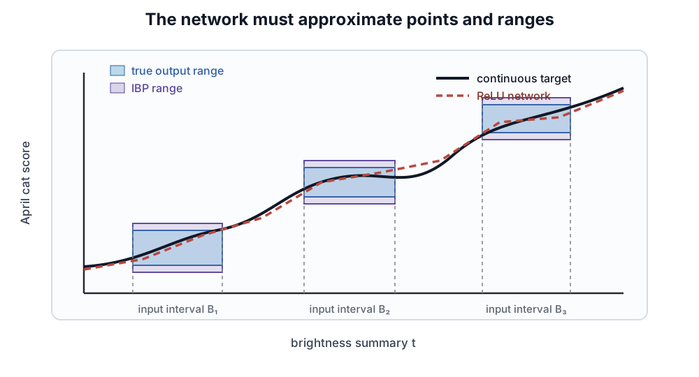
The theorem settles the existence question by allowing us to choose a network adapted to the target and the desired tolerance. A later interval universal approximation theorem extends the existence result from ReLU to a broad family of activation functions.

Can we construct the network that the theorem promises?

The theorem proves that suitable weights exist, but it does not give a practical way to find them. A training algorithm begins with an architecture and initial weights, then searches a high-dimensional parameter space under a finite compute budget. The computational cost of that search is a separate question.

The generalized interval-approximation study makes this gap concrete. Its proof constructs a network by dividing the input domain into a grid. As the input dimension grows, the number of grid regions grows exponentially, so the construction itself can become impractical even though it proves existence.

The paper then isolates a simpler problem. Given a network with outputs in $[0,1]$, approximate its minimum and maximum within an error $\delta<1/2$. Solving this range-approximation problem requires finding values near the extrema and ruling out values beyond them. The paper proves that both directions are hard: the problem is NP-hard and coNP-hard. Under the standard assumption $\mathsf{coNP}\not\subseteq\mathsf{NP}$, the range-approximation theorem classifies it as strictly harder than NP-complete problems. An efficient construction of an interval universal approximator would also solve this range problem, so the hardness transfers to constructing such networks in general.

Universal approximation therefore leaves an algorithmic question:

How do we reliably find compact, accurate networks that IBP can certify?

Certified training provides a practical search strategy for these weights. It chooses an architecture, adjusts its weights using a tractable relaxation of the worst-case loss, and tries to reach a network that IBP can certify. A more precise relaxation seems like a better guide because its loss lies closer to the exact worst-case loss. Frontier 2 asks whether that additional precision actually helps the optimizer find better weights.

Frontier 2: Why can a tighter training bound produce a worse model?

Fix a trained network. Suppose relaxation $A$ always gives a smaller sound upper bound than relaxation $B$ for the violation we want to rule out. Then $A$ is tighter: any case proved safe by $B$ is also proved safe by $A$.

This fixed-network fact suggests a natural training strategy: use the tighter relaxation as the loss because it follows the true worst-case value more closely. Training changes the weights, however, so the comparison at one network does not determine how either loss guides optimization.

Each gradient step changes the weights and therefore changes the next bound. The optimizer must navigate the whole surface

\[\theta\longmapsto L_{\mathrm{cert}}(\theta),\]

where $\theta$ contains all trainable weights. Tightness measures the vertical gap between this certified loss and the exact worst-case loss at one value of $\theta$. Optimization also depends on how the surface changes between nearby weight values.

Empirical results often reverse this expectation. Loose interval-based training can produce networks with higher certified robustness than training with tighter relaxations. This behavior is known as the paradox of certified training.

Towards Better Understanding of Training Certifiably Robust Models against Adversarial Examples studies the paradox through the loss landscape. It identifies smoothness as another factor alongside tightness and finds substantial differences among the landscapes induced by linear-relaxation methods. The paper also designs a method around both criteria and evaluates it across a wide range of perturbation sizes.

On the Paradox of Certified Training develops this optimization view further by separating two properties beyond tightness:

• Continuity: nearby weights should produce nearby bound values. A jump gives the current gradient no information about the landscape across the discontinuity.
• Sensitivity: this describes how algebraically complicated the bound becomes as the weights change. High sensitivity can create high-degree rational loss surfaces with additional local optima and saddle points.

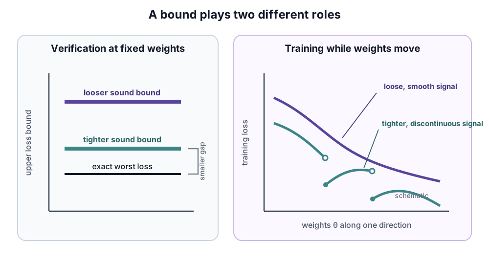
This diagnosis suggests a repair: average the certified loss over nearby weight settings before optimizing it. Gaussian Loss Smoothing defines the averaged loss as

\[L_\sigma(\theta) =\mathbb{E}_{\epsilon\sim\mathcal{N}(0,\sigma^2I)} \left[L_{\mathrm{cert}}(\theta+\epsilon)\right].\]

The random vector $\epsilon$ perturbs every trainable weight. A jump at one weight setting contributes only one value to an average over its neighborhood, so the smoothed loss changes more regularly as $\theta$ moves.

The paper proves that, under a growth condition on the loss as the weights become large, $L_\sigma$ is infinitely differentiable. If optimization stays in a compact parameter region, $L_\sigma$ is also Lipschitz continuous. Its deviation from convexity, a measure of how far the surface bends away from a convex landscape, cannot increase under smoothing. These properties directly address the discontinuity, non-smoothness, and sensitivity diagnosed above.

Computing the expectation exactly would be expensive, so the paper estimates it in two ways. Policy Gradients with Parameter-based Exploration (PGPE) uses only loss evaluations and therefore supports non-differentiable relaxations. Randomized Gradient Smoothing (RGS) averages gradients and is more efficient than PGPE, but it requires a differentiable relaxation. Across many settings with matched network architectures, these methods enable tight relaxations to surpass existing certified-training methods.

At fixed weights, a tighter sound bound remains better for verification. During training, the optimizer must also be able to follow the bound as the weights change. Gaussian loss smoothing demonstrates one way to make tight losses easier to navigate. A useful certified-training objective therefore needs both precision and favorable optimization dynamics.

Training addressed whether an optimizer can find good weights. The next frontier returns to the existence question and raises the standard from approximation to equality: which target functions have an exact network representation that the chosen relaxation can also bound exactly?

Frontier 3: Which functions remain precisely expressible under single- and multi-neuron relaxations?

Fix a target function $f$, a relaxation, and the input regions we want to certify. The precise-expressivity question asks whether there exists a finite ReLU network that computes $f$ exactly and whose relaxation returns the exact output range on every required region. We may choose the architecture and weights to suit the relaxation. The single-neuron study below requires one network to work on every input box. The multi-neuron result later fixes an arbitrary convex region $X$. Both use the same order of choices: specify the target and regions, then search over equivalent network representations.

An inexact bound for one familiar representation therefore does not settle the question. Every equivalent network representation must fail before the function lies outside the precisely expressible class.

This requirement is stronger than Frontier 1. Approximate existence allowed a positive error tolerance in both the predictions and the IBP ranges. Precise expressivity requires zero prediction error and zero bounding error.

Triangle and DeepPoly from Part 4 use a convex relaxation: a tractable convex superset of the network’s exact behaviors. For every unstable ReLU, whose input interval crosses zero, they add linear inequalities that enclose the ReLU graph.

The verifier still retains the shared affine equations between neurons. A single-neuron relaxation derives each nonlinear ReLU envelope only from that ReLU’s scalar input interval. It adds no new inequality coupling the ReLU output to a neighboring value.

Consider the network

\[a=x_1-x_2,\qquad b=x_2,\qquad c=\operatorname{ReLU}(a),\]

with output

\[f=c+b=x_2+\operatorname{ReLU}(x_1-x_2) =\max(x_1,x_2).\]

Let $(x_1,x_2)\in[0,1]^2$. Because $f$ is the maximum of two numbers in $[0,1]$, its exact output range is $[0,1]$.

A single-neuron Triangle relaxation sees only $a\in[-1,1]$ when it relaxes $c=\operatorname{ReLU}(a)$. Its upper line is

\[c\leq\frac{a+1}{2}.\]

At $x_1=x_2=1$, the exact ReLU value is $c=\operatorname{ReLU}(0)=0$. The Triangle constraints also permit the spurious value $c=0.5$. Pairing this value with $a=0$ and $b=1$ makes the relaxed output reach

\[f=c+b=1.5,\]

although the exact network output there is $1$. The envelope is optimal for $c$ as a function of $a$ alone. Its spurious value survives because the envelope does not record how $c$ and $b=x_2$ depend on the same inputs.

This calculation could still leave an architectural escape route: rewrite $\max(x_1,x_2)$ as a different ReLU network whose single-neuron relaxation is exact. Expressivity of ReLU-Networks under Convex Relaxations closes that route. It proves that for every finite ReLU network computing the two-dimensional maximum exactly, Triangle is inexact on some input box. Triangle already uses the tightest convex envelope of each ReLU separately, so no weaker single-neuron convex relaxation can avoid the barrier.

The precise-expressivity boundary depends on the input dimension. For functions of one variable, the same paper constructs suitable Triangle and DeepPoly networks for every convex continuous piecewise-linear target. With multiple inputs, even the convex, monotone function $\max(x_1,x_2)$ lies beyond every single-neuron convex relaxation. This negative result concerns the whole class of equivalent network representations rather than one unlucky encoding.

The natural next question keeps the target function fixed and strengthens the relaxation. Can joint constraints make $\max(x_1,x_2)$ precisely expressible?

Multi-neuron constraints enlarge the precisely expressible class

A multi-neuron relaxation derives constraints for a group of values together. Its ideal form uses their joint convex hull, the smallest convex set containing every exact feasible point. For the same network, this joint reasoning supplies two valid inequalities:

\[c\leq 1-b,\qquad c\leq a+b.\]

Their meaning is visible from the original inputs. Since $x_1\leq1$, we have $c=\max(x_1-b,0)\leq1-b$. Since $x_2\geq0$, we also have $c=\max(x_1-x_2,0)\leq x_1=a+b$. The first inequality immediately gives

\[f=c+b\leq 1.\]

The exact lower bound $f\geq0$ follows from $c\geq0$ and $b\geq0$, so the multi-neuron relaxation recovers the exact range $[0,1]$.

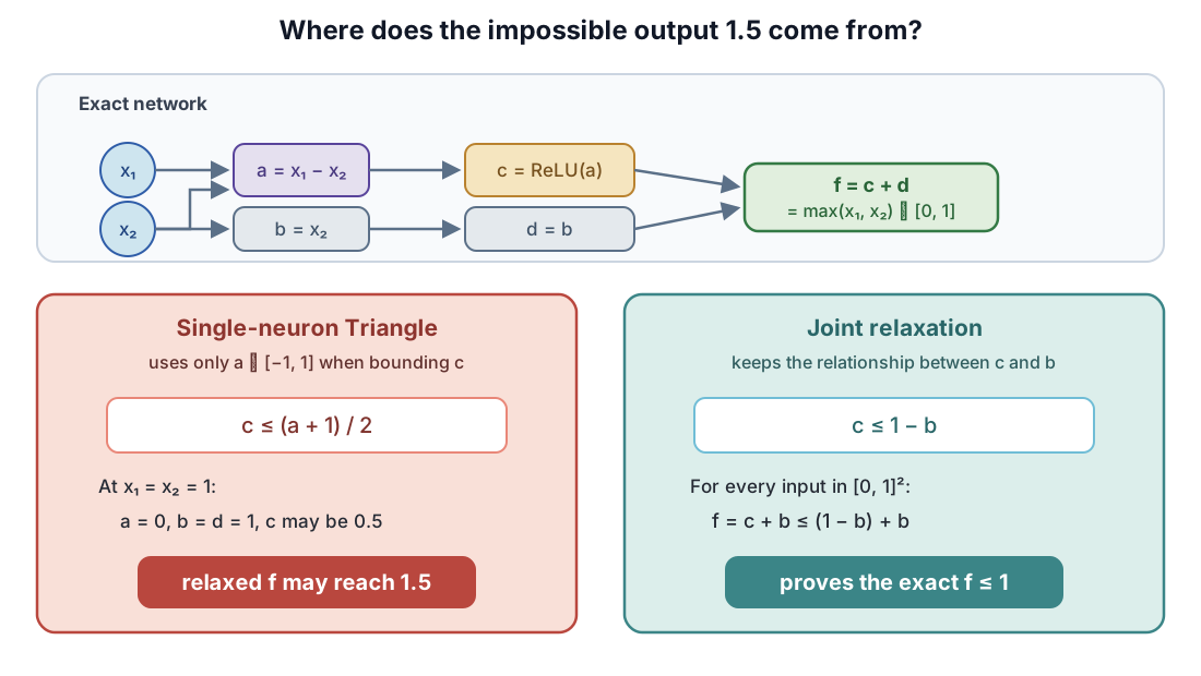
The expressiveness analysis of multi-neuron convex relaxations formalizes this separation. For every continuous piecewise-linear function $f$ and specified convex input region $X$, it proves that a finite ReLU network exists that equals $f$ on $X$ and is bounded exactly there by an optimal layerwise multi-neuron relaxation. The construction widens the network so that copies of the input survive through its hidden layers. The last relaxation then retains enough information to recover the exact output range.

The maximum example needs much less machinery. The two joint inequalities above already recover its exact range on $[0,1]^2$, and the paper extends the construction to $\max(x_1,\ldots,x_d)$ on $[0,1]^d$. Single-neuron relaxations cannot precisely express even the two-input case, while multi-neuron relaxations preserve the full continuous piecewise-linear function class on a specified convex region.

Frontier 3 therefore concerns the existence of a relaxation-friendly network representation. It does not imply that the same multi-neuron relaxation returns exact bounds for every network representation. To ask that stronger question, we must reverse the order of choices: fix an arbitrary network first, then ask the verifier to bound it.

Frontier 4: Can a fixed convex relaxation exactly bound every network?

A verifier is complete when it returns exact bounds for every supported network and input region. Precise expressivity let us redesign the network for the relaxation. Completeness must also handle representations that were chosen without the relaxation in mind.

Frontier 3’s positive result used a layerwise multi-neuron relaxation. At its strongest, it can relate every neuron in one layer, yet it replaces that layer’s reachable set with convex information before moving onward. This leaves a natural escape route: analyze several consecutive layers together.

A cross-layer multi-neuron relaxation opens a window over $r$ consecutive layers and can derive constraints that connect variables inside that window. The strongest possible cross-$r$-layer relaxation computes the exact convex hull of each window’s input-output graph. If this ideal relaxation fails, every cross-$r$-layer convex relaxation also fails.

For example, when $L=5$ and $r=3$, the windows cover layers 1–3, 2–4, and 3–5. Their overlap carries intermediate variables across neighboring windows.

Let a network have $L$ layers. The multi-neuron expressiveness study proves a sharp threshold. Choose any fixed fraction $0<\alpha<1$ and let each window span

\[r=\max(1,\lfloor\alpha L\rfloor)\]

layers. Even the strongest cross-$r$-layer relaxation is inexact on some networks, and its bounding error can be arbitrarily large. The window may span 90% or 99% of the network. Exact bounds for every network appear only at $\alpha=1$, when one convex hull covers the complete input-output function.

This sharp threshold establishes the universal convex barrier across three levels of convex reasoning:

1. a separate relaxation for each neuron;
2. joint constraints over any number of neurons within one layer; and
3. joint constraints across a fixed number of layers, or even any fixed fraction of the network depth below the complete network.

Cross-layer reasoning moves the point where information is convexified farther through the network. For every $\alpha<1$, at least one boundary remains. The paper constructs a failure case by inserting function-preserving identity layers between two subnetworks. These layers push a critical dependency beyond the reach of each cross-layer window.

At that boundary, April’s allowed inputs may reach a non-convex set $S$. Replacing $S$ by its convex hull admits a spurious hidden state $c$. Later layers can map $c$ beyond every output produced by the exact network, so the final relaxed range becomes inexact. The same mechanism applies when the convexified window contains one layer or many layers.

Practical methods such as PRIMA approximate joint convex hulls over small neuron groups within one layer. Cross-layer methods retain relationships through several consecutive layers. Larger groups and deeper windows can tighten many concrete problems. The theorem still covers their ideal counterparts for every fixed window size and every fixed fraction of network depth below 100%.

Two ways to recover exact bounds

The universal barrier assumes that one bounded-scope convex relaxation must analyze the given network and region directly. The study identifies two ways to change that setup:

1. Transform the network. Add carefully designed ReLU neurons that preserve the original function while carrying important input relationships forward. This is the representation change behind Frontier 3’s positive expressivity result.
2. Partition the input. Divide the input region into convex pieces whose reachable sets remain convex through the network, then bound every piece. This reconnects multi-neuron relaxations with the divide-and-conquer method from Part 5.

The nested maximum makes the potential difference concrete. For $\max(x_1,\ldots,x_d)$ on $[0,1]^d$, the paper’s multi-neuron construction needs one subproblem and a number of constraints that grows linearly with $d$. An exact DeepPoly branch-and-bound proof must instead separate all $2^{d-1}$ activation patterns for this construction.

The result leaves a concrete research question:

How should a verifier combine joint constraints, representation changes, and input partitions to reach exact bounds at manageable cost?

Four frontiers, one certification pipeline

The four frontiers differ in both the accuracy they require and which object we are allowed to choose.

Frontier	What may be chosen?	What we learned
Approximate existence	A network adapted to the target and a positive tolerance	IBP-certified networks can approximate every continuous target and its ranges arbitrarily closely.
Trainability	An optimization path through a chosen architecture	Tightness alone does not determine training quality. Continuity and sensitivity also shape the search.
Precise expressivity	A network representation adapted to the target and relaxation	Single-neuron relaxations lose some multivariate functions, while layerwise multi-neuron relaxations preserve the full continuous piecewise-linear class on a specified convex region.
Completeness	The network is already fixed	Layerwise and bounded-scope cross-layer convex relaxations are inexact on some networks. Exactness requires changing the representation or partitioning the input region.

Frontiers 1 and 3 both let us choose a network. Frontier 1 permits an arbitrarily small positive error, while Frontier 3 requires exact equality. Frontier 4 fixes the network before verification. Training connects these existence results to practice by asking whether optimization can reach the promised representations. Keeping these choices in order prevents a positive result at one frontier from answering a different question.

Every certificate so far has propagated deterministic bounds over an allowed input region. Part 8 takes a probabilistic route: add random noise, measure how often April’s label wins, and convert that probability into a certified radius.